So what is it that derivative is supposed to help accomplish?  Most of us get by most of the time with simply using the “P” and “I” components when tuning a loop and if the loop is reasonably fast such as a flow meter or speed adjustment or even pressure we can get the job done and not have to deal with derivative.

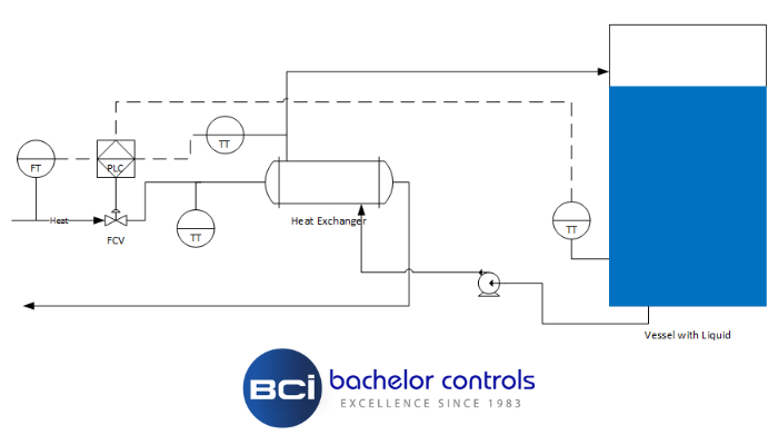
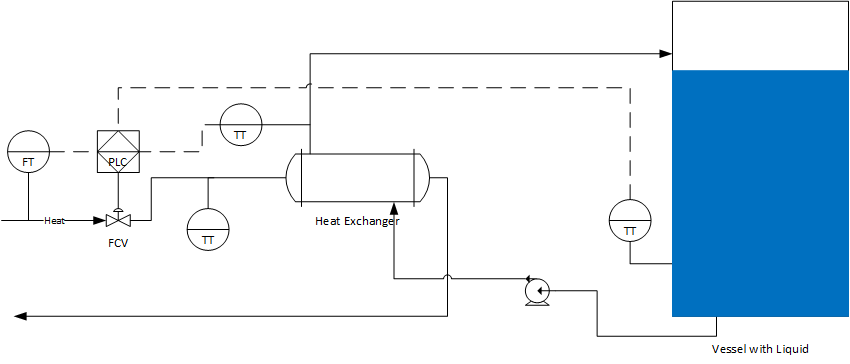
When we’re dealing with loops that have long response times such as temperature loops for tanks or dryers, there is a tendency to over-damp those loops to avoid massive overshoot of the process variable (that is if you don’t use the derivative component).

If we just think about our car for a minute, let’s pretend that we are the PID loop control and the speedometer is our process variable and the speed limit (hopefully) is the setpoint. If we only use “P” to govern how we apply the accelerator then we’ll never reach setpoint because “P” needs some error in order to have an output and since this is a linear direct proportion (gain being the proportionate factor) it is also immediately responsive.  You would get a lot of accelerator when the car was first at zero speed and then as the speed increased the accelerator would be decreased in proportion to the difference between the current speed and the desired speed (setpoint).  Well, we don’t want to have a setpoint in mind of 80 mph (western Nebraska) and only be going 50 mph.

So we need to incorporate something that continues to add to the accelerator as long as there is an error.  Since this error is measured algebraically and we are below the desired speed we need to determine how much we continue to add every time we look at the speedometer in order to reach our desired speed (integral component).

This integral component needs to know how often we’re going to look at the speedometer and how much we’ll add as a function of how far we are from the desired speed (setpoint).  Of course the closer we get to the speed the less proportional correction we have so we have to keep adding the integral component in order to make up for that difference and continue to increase our speed.

As we get closer and closer to the desired speed the entire accelerator action is the result of the integral addition – remember that with no error (desired minus actual) there is no proportional contribution.

So all is well until we reach the desired speed. By now we’re shoving down the accelerator pretty aggressively (remember that the integral can’t reduce its contribution until the algebraic sign changes (speed goes over desired setpoint).  So here we are zooming down the highway and the only thing we have available to us for adjusting our speed down is again the integral, but once we blow past the setpoint (speed limit) we now have a change in the algebraic value – the integral will subtract its contribution in accordance with the same proportion and time interval that was used to increase the accelerator.  So you can see that not a great deal is going to happen to reduce speed the moment we blow past the setpoint. Until we have some measurable error on the other side of the setpoint not much is going to change at the gas pedal.

Wouldn’t it be nice if we had some way of knowing that we should be backing off the accelerator a little bit prior to blasting through the setpoint.  Yes, we know we are getting close to the setpoint with just “P” and “I” and make the contributions smaller as we get closer (nevertheless those contributions are still additive). What we don’t know is how fast we are closing in on the speed target. It would be helpful to have something that could help us understand that we are approaching the setpoint way too aggressively and need to start backing off before we get there?

This is where derivative comes in. What the derivative component does is look at rate of change. Remember that integral is adding less and less as we approach the setpoint, but it is still additive.  We need something (derivative) to be removing some contribution as a result of rate of change. Its job is to start slowing down the closure rate (back off the accelerator a little) before you get there.  As it removes some accelerator then the rate of change reduces so that the next time it looks at the speedometer, it removes less than the time before, etc.

The idea is once you have reached setpoint the derivative contribution is now zero along with the proportional contribution and the total contribution is now attributable to the integral component.

I acknowledge that this “speedometer” story is a simplistic example, but I also feel that we sometimes over-think this PID tuning issue and get lost in the process.

I should point out that not all loops can be successfully tuned using PID e.g. if they are improperly designed mechanically. There is a mechanical gain in the system that adds to the complexity as well not to mention mechanical lag (slop in a mechanical linkage) or uneven mechanical gain (binding).

As an example, if the control valve is so large for the required steady state flow that steady state is a barely open condition then the mechanical gain of the system is too high and something needs to be adjusted mechanically in order to allow the control algorithm to accomplish its task. Unstable sensor feedback is another factor that will make tuning a PID difficult if not impossible. There are other examples, but the essence of the story is to help people think through what derivative is intended to do and not be afraid to apply it when needed. The only other PID option to limit overshoot is to simply over-damp the loop until it sluggishly reaches setpoint and then sluggishly corrects.

This article is for general information purposes only and should not be relied upon for any particular engineering solution.

Ray Bachelor
Chairman of the Board

Download:  Why the Derivative